Derivation of the 1-D Heat Equation and Basic Numerical Methods
When I took a course in Large Scale Computation at Tulane University, I learned a lot and forgot a lot. Understanding how to take a physical phenomena or problem and develop software that is scalable and highly parallelizable, along with optimizing the software for the High Performance Computing (HPC) resources available is enough information to justify a whole degree, so trying to learn all of that in the semester courses that are taught on HPC (if at all) can feel like drinking water from a fire hose. In going back over the class notes I re-remembered one of problems that encompasses all the important parts for scientific computing on HPC resources and in relearning it felt like it would be a great example for beginners to work through.
Heat equation
The heat equation is one of the most well known and simplest partial differential equations (PDEs). The physical intuition and solving the heat equation provides the fundamentals for other equations throughout mathematics and physics. The heat equation and other diffusive PDEs show up throughout statistical mechanics describing random walks and Brownian motion. While the heat equation in 1-D and some other PDEs have analytical solutions, solving most PDEs requires numerical methods to solve.
In this first part of a multi-part series using the example of heat flow in a uniform rod, we’ll go over the physical interpretation of the heat equation, mathematical setup, and discretization for the numerical solution. In later parts of the series we’ll use C++ and open-source parallel computing libraries to solve the problem numerically on HPC resources.
Physical interpretation
From the second law of thermodynamics heat flows from hot to cold proportional to the temperature difference and the thermal conductivity of the material between them. This provides the intuitive result that the rate of heating or cooling is proportional to how much hotter or cooler the surrounding area is.
Conservation of heat
 is some conserved quantity,
  is a source term, and
  and
and  are the flux at
  and
and  , respectively.
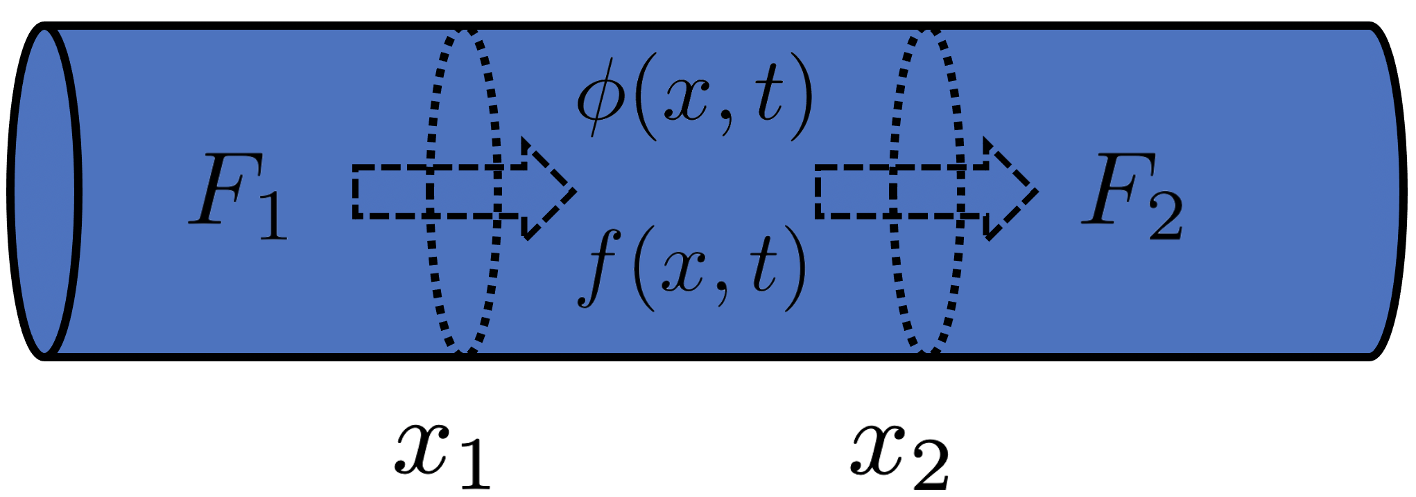
Here we have a conserved quantity, where  might be heat or mass. The total amount of this conserved quantity in an interval
  is defined as,
(1) 
To describe how the amount changes with time over the same interval,
(2) 
Because is a conserved quantity, Eq. (2) has to balance with the flux at the boundaries, and , and the generation/consumption term within the interval,
(3) 
Using Fick’s Law, the flux is proportional to the gradient,  , where
  is a constant related to the diffusivity of the material. Using Fick’s Law with Eq. (3),
![\begin{equation*} \frac{d}{dt} \int_{x_1}^{x_2} \phi (x,t) d x = -\left[-\mathcal{D} \frac{\partial}{\partial x}\phi (x,t) \right ]^{x_2}_{x_1}+ \int_{x_1}^{x_2}f(x,t) d x \implies \end{equation*}](https://www.diegogomez.studio/wp-content/ql-cache/quicklatex.com-9b553ed19261039e21e96a80cee3419f_l3.png "Rendered by QuickLaTeX.com")
(4) 
Leibniz integral rule
Using the Leibniz integral rule, we can differentiate under the integral sign of the left side of Eq. (4). The Leibniz integral rule states that for a multivariate function (here is a function of  and
and  and not the generation/consumption term related to the physical problem) on the interval
  the derivative of the integral
  can be expressed as,

Often the above simplifies into,

Because the boundary conditions,  and
and  are constants and their derivative will be 0.
Final formulation
Applying the Leibniz integral rule with Eq. (4),
(5) 
And because all terms of Eq. (5) have the same limits of integration and same differential it can be simplified to,
(6) 
Steady-state with Dirichlet boundary condition
For steady-state the time derivative of is zero, the equation can be reduced to,
(7) 
With the Dirichlet boundary conditions of  and
and  .
.
Finite difference method
To evaluate the steady-state heat equation numerically, Eq. (7) must be discretized. This is done approximating the derivative  evaluated at a point
  to a finite difference between the two nodes outside of the derivative being approximated,
  and
and  , and the “infinitesimal” distance between the two nodes
  .
.
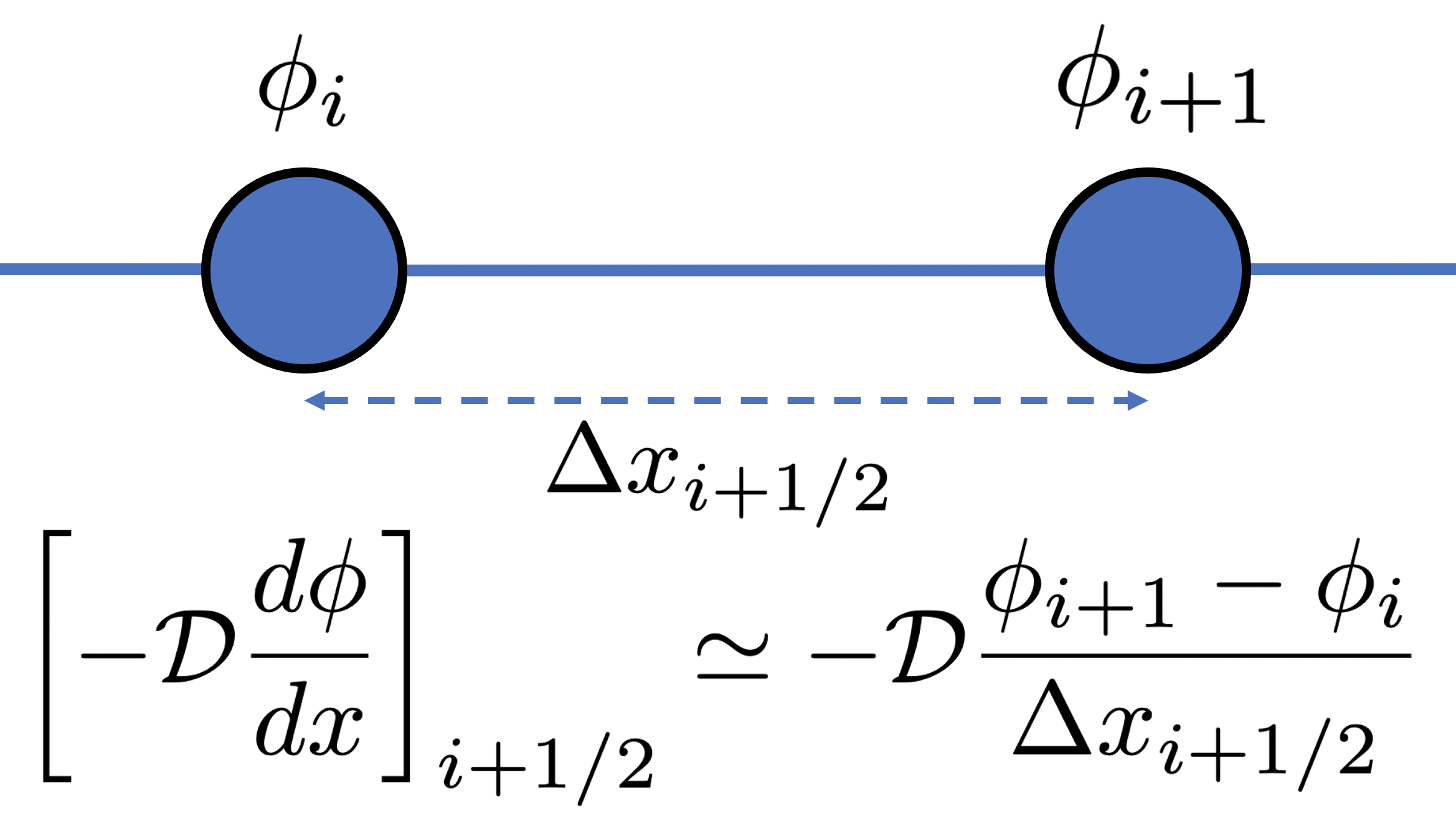
![\left [ -\mathcal{D} \frac{d \phi}{d x} \right ]](https://www.diegogomez.studio/wp-content/ql-cache/quicklatex.com-fed9ac3450130e3ebea5a7e559172055_l3.png "Rendered by QuickLaTeX.com") evaluated at can be approximated by difference between and divided by the spacing between the s, .
evaluated at can be approximated by difference between and divided by the spacing between the s, .Again using Fick’s Law, the flux is equal to the gradient, we can now use the central difference by substituting the flux,  , into Eq. (7),
(8) 
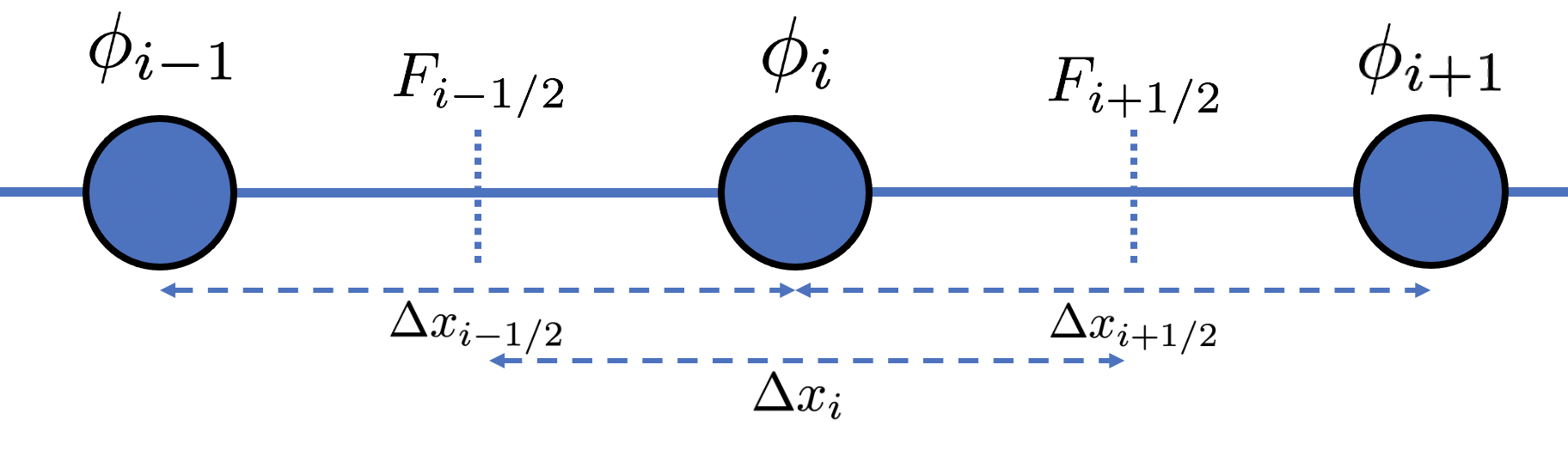
The central difference of the flux,
![\begin{equation*} -\left [ \frac{d F}{d x} \right ]_{i} \simeq - \frac{F_{i+1/2} - F_{i-1/2}}{\Delta x_i} \end{equation}](https://www.diegogomez.studio/wp-content/ql-cache/quicklatex.com-28a3dda3c182d60585f8630b29629bcb_l3.png "Rendered by QuickLaTeX.com")
And since,
![\begin{equation*} F_{i+1/2} = \left [ -\mathcal{D} \frac{d \phi}{d x} \right ]_{i+1/2} \simeq -\mathcal{D}\frac{\phi_{i+1} - \phi_{i}}{\Delta x_{i+1/2}} \end{equation*}](https://www.diegogomez.studio/wp-content/ql-cache/quicklatex.com-559d06de7158a946620604e887b5c0ed_l3.png "Rendered by QuickLaTeX.com")
and,
![\begin{equation*} F_{i-1/2} = \left [ -\mathcal{D} \frac{d \phi}{d x} \right ]_{i-1/2} \simeq -\mathcal{D}\frac{\phi_{i} - \phi_{i-1}}{\Delta x_{i-1/2}} \end{equation*}](https://www.diegogomez.studio/wp-content/ql-cache/quicklatex.com-4d2d5804c6068e79d28e81f56221e6e4_l3.png "Rendered by QuickLaTeX.com")
The discrete form of Eq. (8) is,
(9) ![\begin{equation*} \frac{\mathcal{D}}{\Delta x_i}\left [ \frac{(\phi_{i+1}-\phi_i)}{\Delta x_{i+1/2}} - \frac{(\phi_{i}-\phi_{i-1})}{\Delta x_{i-1/2}} \right ]+ f(x_i) = 0 \end{equation*}](https://www.diegogomez.studio/wp-content/ql-cache/quicklatex.com-2b91c343cbf41459094d56c390c55676_l3.png "Rendered by QuickLaTeX.com")
And if  and
and  is uniform Eq. (9) simplifies into,
(10) 
Numerical grid and linear system
Consider a uniform grid within  ,
,

In this example, the uniform grid has 7 node points and including the boundary conditions the value of must satisfy the the following linear system of equations,

This system of linear system of equations in Matrix-Vector form,
(11) 
This forms the classic Matrix-Vector equation
(12) 
Where  is a matrix, and both
  and
and  are vectors. Through matrix algebra, can be solved for by computing
  .
.
For HPC, and scientific computations in general, it is beneficial for to be a symmetric matrix. In Eq. (11), the matrix is close to being symmetric and we can take advantage that  and
and  are known but are included in the unknown vector . By eliminating and from the system of linear equations and the matrix in Eq. (7),

Resulting in,
(13) 
And now is symmetric. Now that we have our physical problem discretized, and setup in such a way that in  , is symmetric we can begin to solve numerically.
Iterative method
When solving for the unknown vector, , from the linear system of equations from Eq. (12), is solved with iterative methods, using the sceme,
(14) 
Where  and
and  are unknown constant vector matrix and vector and
  is a step that may not satisfy the equation Eq. (12) and
  is the iterative step counter. We begin to solve for , the solution must satisfy the equation,
![\[\mathbf{x}=\mathbf{B}\mathbf{x} + \mathbf{c}\]](https://www.diegogomez.studio/wp-content/ql-cache/quicklatex.com-06eb903f0b0c404f98598dd396882dd9_l3.png "Rendered by QuickLaTeX.com")
Solving for and using the ,
![\[\mathbf{c}= (\mathbf{I} - \mathbf{B})\mathbf{A}^{-1}\mathbf{b}\]](https://www.diegogomez.studio/wp-content/ql-cache/quicklatex.com-338b9282552b249d00721cc2321485c6_l3.png "Rendered by QuickLaTeX.com")
The iterative scheme of Eq. (14) is now,
(15) 
Where  and
and  . can be split as,
(16) 
We arrive at the final equation for computing the unknown vector  is,
is,
(17) 
For an iterative method, computing  and
and  must converge rapidly and be computationally inexpensive.
Convergence
The error for an iterative method at step is  . The error must also satisfy the equation,
(18) 
And converges if,
![\[\lim_{k \to \infty}=\mathbf{e}^k=0\]](https://www.diegogomez.studio/wp-content/ql-cache/quicklatex.com-81d4af9b2be6a657aeb551ca407131af_l3.png "Rendered by QuickLaTeX.com")
Also assuming that  has the eigenvalue equation,
(19) ![\begin{equation*} \mathbf{B}\mathbf{z}_i = \lambda_i \mathbf{z}_i \qquad i = 1,\cdots,\mathrm{rank}\left [ \mathbf{B}\right ] \end{equation*}](https://www.diegogomez.studio/wp-content/ql-cache/quicklatex.com-7a9d4e102dc5a1a033431c0357329bb5_l3.png "Rendered by QuickLaTeX.com")
The initial error,  using the eigenvectors from Eq. (19) is defined as
(20) ![\begin{equation*} \mathbf{e}^0 := \sum_{i=1}^{\mathrm{rank}\left [ \mathbf{B}\right ]} a_i \mathbf{z}_i \end{equation*}](https://www.diegogomez.studio/wp-content/ql-cache/quicklatex.com-48f11d62b8a488d99d88b83dc8551dc1_l3.png "Rendered by QuickLaTeX.com")
Where  is a constant. Resulting in the formula for
  ,
,
(21) ![\begin{equation*} \mathbf{e}^k = \sum_{i=1}^{\mathrm{rank}\left [ \mathbf{B}\right ]} a_i (\lambda_i)^k \mathbf{z}_i \end{equation*}](https://www.diegogomez.studio/wp-content/ql-cache/quicklatex.com-8c2932cd4a60c388cf4a03ac4fdec38b_l3.png "Rendered by QuickLaTeX.com")
If the magnitude of the eigenvalues,  is less than 1, converges to 0 as
  . For convergence the spectral radius of ,
  , must meet the criteria,
(22) 
For the matrix from Eq. (12) to have guaranteed convergence the following criteria must be met,
(23) 
Jacobi Method for the 1-D heat equation
The simplest iterative method is the Jacobi Method. An  matrix has a matrix
  composed of the diagonal elements of ,
![\[\mathbf{D}=\mathbf{A}_{ii}\]](https://www.diegogomez.studio/wp-content/ql-cache/quicklatex.com-b6299245c2ba19343ae5425481098ad0_l3.png "Rendered by QuickLaTeX.com")
Computing only inverse of the diagonal elements is fast and easy, resulting in,  . We will define
  as the off-diagonal elements of
  ,
,
![\[\mathbf{N}=-\mathbf{A}_{ij} \qquad i \ne j\]](https://www.diegogomez.studio/wp-content/ql-cache/quicklatex.com-06a503b1dad66b936ff76a536f849ca8_l3.png "Rendered by QuickLaTeX.com")
For any iterative method to have guaranteed convergence the spectral radius must follow Eq. (23). The Jacobi Method also provides another sufficient condition of convergence that is,
(24) 
The matrix from Eq. (13), is clearly diagonally dominant so our unknown vector will converge as . The diagonal matrix ,

And from Eq. (16)  has the off-diagonal elements of ,

The iterative scheme solving for solving  from Eq. (13) is now,
(25) 
And where is the number of iterations. The last term for Eq. (17) is,
(26) 
For the Jacobi Method, the general equation to find at node  after
after  steps is using the matrix is,
(27) 
Gauss-Seidel Method
The Gauss-Seidel method is another iterative method. The main difference between Gauss-Seidel and the Jacobi method is that the diagonal matrix, , is determined by the lower triangle elements of in Gauss-Seidel is the,
(28) 
And now the matrix contains the upper triangle elements of ,
(29) 
Similar to the Jacobi Method, if the matrix is diagonally dominant, Gauss-Seidel converges from Eq. (24).
Solving the 1-D heat equation’s linear system of equations from Eq. (13) the matrices for Gauss-Seidel become,

and,

The iterative scheme is again Eq. (17). For Gauss-Seidel the computation for is more involved than for the Jacobi method. Our system is,

And now,

The linear system of equations becomes,

We can solve the general form for  using induction. The first term,
  is,
is,
![\[\phi_1^{k+1}=\frac{c_1}{D_{11}}\]](https://www.diegogomez.studio/wp-content/ql-cache/quicklatex.com-8ab3614d17d638658f2be58695292c49_l3.png "Rendered by QuickLaTeX.com")
The second term,  ,
,

And the third term,

And finally for the th node at the step the general equation is,
(30) 
Next in the series
In future posts of this series, we’ll solve this problem numerically using C++ with OpenMP and MPI!