Paul Ehrenfest

Paul Ehrenfest is one of premier statistical mechanics of all time. Following in the footsteps of his advisor, and the father of statistical mechanics, Ludwig Boltzmann, Ehrenfest was renowned for his focus and clarity on fundamental problems.

The Ehrenfest Model

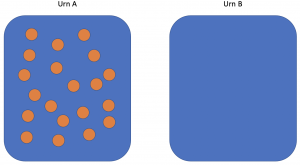
The Ehrenfest model, sometimes called the urn model or the dog-flea model, is a simple, discrete model for the exchange of gas molecules between two containers.

Consider two urns, A and B. Urn A contains $k$ marbles and urn B contains none. The marbles are labelled $1,2,...k$ . In each step of the algorithm, a number between 1 and $k$ is chosen randomly, with all values having equal probability. The marble corresponding to that value is moved to the opposite urn. Hence the first step of the algorithm will always involve moving a marble from A to B.

To begin, the Markov chain will need to be defined. Define the random variable $X$ as the number of balls in urn A and the state space $\mathcal{S} \in \{0,1,2,...,k\}$ and the probability of $i$ balls in urn A at step $n$ $P(X_n = i)$ .

The transition matrix looks:

$P= \begin{blockarray}{cccccccccc} & 0 & 1 & 2 & 3 & \ldots & k-2 & k-1 & k\\ \begin{block}{c(cccccccc)} 0 & 0 & 1 & 0 & 0 & \ldots & 0 & 0 & 0 \\ 1 & \frac{1}{k} & 0 & \frac{k-1}{k} & 0 & \ldots & 0 & 0 & 0 \\ 2 & 0 & \frac{2}{k} & 0 & \frac{k-2}{k} & \ldots & 0 & 0 & 0 \\ 3 & 0 & 0 & \frac{3}{k} & 0 & \ldots & 0 & 0 & 0 \\ \vdots & \vdots & \vdots & \vdots & \vdots & \ddots & \vdots & \vdots & \vdots \\ k-2 & 0 & 0 & 0 & 0 & \ldots & 0 & \frac{k-(k-2)}{k} & 0\\ k-1 & 0 & 0 & 0 & 0 & \ldots & \frac{k-1}{k} & 0 & \frac{1}{k}\\ k & 0 & 0 & 0 & 0 & \ldots & 0 & 1 & 0 \end{block} \end{blockarray}$

An important question for the Ehrenfest model is “what is the long term probability that there are $j$ balls in Urn A”.

Stationary distribution using induction

Let, $\boldsymbol{\pi} = (\pi_0,\pi_1,...,\pi_k)$ , be the stationary distribution and $\pi_i$ is the long term probability of $i$ balls in urn A. The three fundamental equations for finding a stationary distribution are,

(1) $\begin{equation*} \pi_j = \sum_{i=0}^N \pi_i P_{ij} \end{equation*}$

(2) $\begin{equation*} \sum_{i=0}^N \pi_i = 1 \end{equation*}$

and,

(3) $\begin{equation*} \boldsymbol{\pi} \boldsymbol{P} = \boldsymbol{\pi} \end{equation*}$

For this problem there’s an easy way to solve it using the fact that $\boldsymbol{xP} = \boldsymbol{x}$ and that $\boldsymbol{x}$ is a vector of the same state space $\boldsymbol{\pi}$ , but not necessarily a probability vector, and that $\boldsymbol{\pi}=c\boldsymbol{x}$ , where $c$ is a constant and $c=\frac{1}{\sum_j x_j}$ . Plainly, instead of solving for $\boldsymbol{\pi}$ we can solve a simpler (hopefully) vector and multiply by a constant later.

Let, $\boldsymbol{x} = (x_0,x_1,...,x_k)$ , then

(4) $\begin{equation*} x_j = \sum_{i=0}^k x_i P_{ij} \end{equation*}$

and $x_0 = 1$ . Because $x_j$ depends only on $x_{j-1}$ and $x_{j+1}$ , and using the probabilities from the transition matrix equation (4) becomes,

(5) $\begin{equation*} x_j = x_{j+1} \frac{k-(j-1)}{k}+ x_{j-1}\frac{j+1}{k} \end{equation*}$

for, $j = 1,2,...,k-1$ , starting with $x_0 = x_1 \frac{1}{k}$ and since $x_0 = 1$ , $1 = x_1\frac{1}{k} \implies x_1 = k$ . Solving equation (5) using the result of $x_1 = k$ starting with $j=1$ ,

$\begin{eqnarray*} x_1 = x_0 \frac{k-(1-1)}{k} + x_2 \frac{1+1}{k} \implies \\ k = 1 + x_2 \frac{2}{k} \implies \\ x_2 = \frac{k(k-1)}{2} \end{eqnarray*}$

$j=2$ ,

$\begin{eqnarray*} x_2 = x_1 \frac{k-(2-1)}{k} + x_3 \frac{2+1}{k} \implies \\ \frac{k(k-1)}{2} = (k-1) + x_3 \frac{3}{k} \implies \\ x_3 = \frac{k(k-1)(k-2)}{6} \end{eqnarray*}$

The pattern is clearly

(6) $\begin{equation*} x_j = \frac{k(k-1)(k-2)\cdots(k-(j-1))}{j!} = {k \choose j} \end{equation*}$

$\boldsymbol{x}$ is known, $c$ can be solved for,

(7) $\begin{equation*} c = \frac{1}{\sum_i x_i} = \frac{1}{\sum_i {k \choose i}} = 2^{-k} \end{equation*}$

using the fact that $\boldsymbol{\pi}=c\boldsymbol{x}$ ,

(8) $\begin{equation*} \pi_j = {k \choose j} 2^{-k} \end{equation*}$

Final thoughts

The max $\pi_j$ is when $j=\frac{k}{2}$ . The Ehrenfest model relates to diffusion of matter and heat, intuitively, objects reach some sort of equilibrium but the importance of Ehrenfest model is that there are still fluctuations between all $\boldsymbol{\pi}$ .

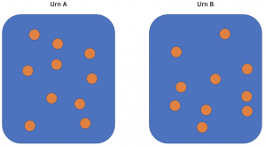
For example, in the $k=20$ case you would expect for the long term probability to be peaked at $j=10$

With no surprise, the long term probability of the two urns have 10 marbles in each.

Long term probability of $k=20$ marbles, where both urns contain $\frac{k}{2}$

As with ergodic systems, there are fluctuations, between the states of $j$ , as $j$ increases, the probability of have less of a variance. When $k=1000$ , $k$ becomes very sharply peaked

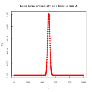Where $k=1000$ , $\pi_j$ becomes sharply peaked.

This example should always be appreciated as a basic and straight forward way for the distribution of microstates in physical systems. Large systems ( $N\approx 10^{10}$ particles, or marbles) become difficult for physical intuition. Paul Ehrenfest, being steeped in the fundamentals of statistical mechanics, knew that systems in equilibrium have a low probability. For instance, the probability of $\pi_0$ is $9.332636\cdot 10^{-302}$ . To put into perspective, there are $8.065818\cdot 10^{67}$ possible decks of cards. The reader has better odds of guessing the order of 5 fully shuffled deck of cards than the long run probability of the Ehrenfest model being in state $j=0$ , i.e. all the marbles being in urn A.

Mark Kac called it “one of the most instructive models in the whole of physics” and to me there is no better example of the sharp distributions of physical systems in equilibrium, and sharp distributions being essential mathematical representation of statistical mechanics.

The Ehrenfest Urn Model

Paul Ehrenfest

The Ehrenfest Model

Stationary distribution using induction

Final thoughts

Leave a comment Cancel reply